How I Built an Offline Photo Geocoding Engine That Clusters 8,000 Photos in Under 5 Seconds
Replacing Apple CLGeocoder with embedded GeoNames data, a K-D Tree, and a chain expansion algorithm to geocode and cluster thousands of photos offline in seconds.
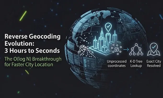
Apple’s CLGeocoder takes 1.3 seconds per request and is rate-limited to 50 requests per minute. For a photo organizer that needs to geocode thousands of photos and cluster them into trips by city, this meant waiting nearly 3 hours. So I replaced it with an embedded geographic database, a K-D Tree, and a chain expansion algorithm - all running offline in seconds.
This article covers every engineering decision: why brute force doesn’t work, how a spatial tree turns O(N) into O(log N), why “nearest city” isn’t enough, and how a chain algorithm captures an entire 5-day trip from a single seed photo.
The Problem With CLGeocoder
Apple provides CLGeocoder for reverse geocoding - converting GPS coordinates to city names. It works, but:
- Rate limited: 50 requests per 60 seconds, with a mandatory 1.3-second delay between calls
- Max ~45 calls per session: After that, requests silently fail
- Network dependent: Every call is a round-trip to Apple’s servers
For a library with 8,000 photos producing 500+ event clusters, this meant 45+ seconds of geocoding with a two-phase UI approach (show placeholder names, then progressively resolve real ones). Users saw “Loading…” for nearly a minute. Unusable.
The Solution: Embedded GeoNames + K-D Tree
The Dataset
GeoNames is an open geographic database. I use cities1000.txt - 167,000 cities worldwide with population > 1,000. After trimming to only needed columns (name, latitude, longitude, country code, population), it compresses to a ~6MB TSV file embedded in the app bundle.
Why cities1000 and not cities15000 (33K cities, pop > 15K)? The smaller dataset missed real cities. Bujanovac, Serbia (~18K residents) wasn’t in it. Neither was Obiliq, Kosovo (12K). Photos in these cities resolved to the nearest larger city - often wrong. The 5x increase in dataset size (1.2MB → 6MB) is worth correct results worldwide.
The K-D Tree: O(log N) Instead of O(N)
A brute-force scan of 167K cities for the nearest one is O(N) per photo. With 8,000 photos, that’s 167K × 8K = 1.3 billion distance calculations. Even at nanosecond speeds, this takes seconds.
A K-D Tree (K-Dimensional Tree) partitions the 2D coordinate space into a binary tree. Finding the nearest neighbor takes O(log N) - about 17 comparisons instead of 167,000. Geocoding all 8,000 photos takes a few seconds total.
I use Bersaelor’s KDTree Swift library, embedded directly in the package (no external dependency). Each city conforms to KDTreePoint with latitude/longitude as dimensions and Haversine distance for squaredDistance:
struct GeoCityPoint: KDTreePoint {
    static let dimensions = 2

    func kdDimension(_ dimension: Int) -> Double {
        dimension == 0 ? latitude : longitude
    }

    func squaredDistance(to other: GeoCityPoint) -> Double {
        let dist = GeoUtils.distanceInKm(
            lat1: latitude, lng1: longitude,
            lat2: other.latitude, lng2: other.longitude
        )
        return dist * dist
    }
}
The tree is built once at initialization (~100ms for 167K cities) and is immutable - no synchronization needed for concurrent reads.
Why “Nearest City” Isn’t Enough: The Suburb Problem
Pure nearest-neighbor geocoding produces results like “Lurup, Germany” instead of “Hamburg, Germany.” Lurup is a Hamburg district - its city center is closer to the photo’s coordinates than Hamburg’s center, so the K-D Tree returns it. But no user wants to see “Lurup” when they were in Hamburg.
The opposite problem exists too: Ferizaj (60K pop, standalone city) is 33km from Pristina (550K). A naive “pick the biggest city nearby” approach would incorrectly label Ferizaj photos as Pristina.
And a third edge case: GeoNames has bad population data for many small cities. Bujanovac shows population 0 despite having ~18K residents. A population-based heuristic would let Vranje (56K, 15km away) absorb it.
The Three-Layer Heuristic
The solution uses three checks:
- Distance: Only consider a parent city within 20km (suburbs are typically < 20km from city center)
- Population ratio: The parent must have 3x the population of the nearest city
- Metropolis threshold: Only cities with population > 100K can absorb neighbors
The metropolis threshold is the key insight. It prevents small cities from absorbing each other regardless of population data quality. Only genuine metropolises (Hamburg, Pristina, Istanbul) absorb their suburbs. Two small neighboring cities always stay independent.
Coordinate-Quantized Cache
Photos taken at similar locations resolve to the same city. A cache keyed by quantized coordinates (~110m grid) avoids redundant suburb detection. For 200 Hamburg photos, only ~50 unique grid cells exist - 150 cache hits save nearestK(30) + distance calculations each.
Smart Clustering: From Photos to Events
Geocoding gives us city names. But we also need to group photos into discrete events - “Hamburg, May 9–12” and “Hamburg, June 3–5” should be separate trips, not one giant bucket.
Phase 1: Time + Distance Splitting
Photos are sorted by date and walked sequentially. A new cluster starts when:
- Time gap to previous photo > 6 hours, OR
- Distance to previous photo > 50 km
This naturally separates morning photos from evening photos (6h gap) and different cities visited the same day (50km distance).
Phase 2: Same-Location Merging
Consecutive clusters at the same quantized location (~111km grid) within 48 hours merge. This reconnects a multi-day stay: Day 1 Hamburg, sleep (6h gap), Day 2 Hamburg → one cluster.
Phase 3: Post-Geocoding Merge
After geocoding, clusters with the same resolved city name within 48h merge. Two clusters at different Hamburg coordinates both geocode to “Hamburg, Germany” → one event.
Phase 4: Chain Rebuild with City Verification
This is the critical step. After geocoding determines cluster names and anchor coordinates, each cluster’s photo set is rebuilt using a chain algorithm:
- Use the city center coordinates as the anchor (not a random photo’s GPS - prevents border-area photos from pulling in neighboring cities)
- Find all library photos within 50km of the city center
- Verify each photo geocodes to the same city name - a photo 45km from Hamburg center that’s actually closer to Bremen gets rejected
- Chain with 24h gap (explained below)
- Sweep no-GPS photos within the established date range
The city-name verification is the key insight that prevents cross-city contamination. Without it, Pristina photos were appearing in Vranje events because they were within 50km of Vranje’s cluster anchor.
The Pre-Computed Dictionary Optimization
The naive approach - calling nearestCity() for each photo in each cluster’s filter - is O(photos × clusters × log N). With 8K photos and 500 clusters, that’s 4 million K-D Tree lookups.
Instead, I pre-compute a [localIdentifier: cityDisplayName] dictionary for ALL GPS photos once:
8,000 photos × O(log 167K) = ~8,000 lookups ≈ 100ms
The per-cluster filter then does a dictionary lookup - O(1). Total: O(M log N) pre-compute + O(M) per cluster, instead of O(M × C × log N). This turned a 30-second freeze into a 100ms operation.
Chain Expansion: Capturing Entire Trips
The original implementation used a fixed ±12-hour window around each event photo. Upload one photo from a 5-day Hamburg trip → only photos within 12 hours matched. 45 out of 163. Wrong.
The Algorithm
Chain expansion works like a flood fill on the time axis:
- Start with seed photos (event photo timestamps) marked as “included”
- Forward pass: Walk the sorted timeline. If photo N is included and photo N+1 is within 24 hours → include N+1
- Backward pass: Same, expanding left
Each newly-included photo extends the chain. A 5-day trip where you took at least one photo per day chains together entirely from a single seed.
No-GPS Photo Sweep
After the chain establishes the trip’s date range using GPS-confirmed photos, a final sweep includes photos without GPS (WhatsApp images, saved files, screenshots) that fall within that window. These couldn’t pass the location filter (no coordinates to verify), but they’re temporally anchored to the trip. The screenshot toggle controls whether screenshots are included in this sweep.
Seed: May 9 21:17 (Hamburg port photo)
Chain forward:  May 9 → May 10 → May 11 → May 12 (no 24h gaps)
Chain backward: May 9 → May 9 14:22 (arrival photos)
Result: May 9 14:22 to May 12 13:17 - entire trip captured
Performance Summary
| Operation | Complexity | Real-world time |
|---|---|---|
| K-D Tree build (167K cities) | O(N log N) | ~100ms (once) |
| Single geocode lookup | O(log N) | ~0.01ms |
| Pre-compute city names (8K photos) | O(M log N) | ~100ms |
| Per-cluster chain filter | O(M) dict lookup | <1ms |
| Full pipeline (8K photos → 500 events) | O(M log N + M×C) | ~2–5 seconds |
Compare to CLGeocoder: 45+ seconds for 45 lookups, then you’re rate-limited.
The SDK
The entire engine is extracted into a reusable Swift Package - GeoClusteringSDK. Zero external dependencies. Zero network calls. Fully offline.
All parameters are configurable:
import GeoClusteringSDK

let sdk = GeoClusteringService()
let events = await sdk.clusterItems(itemMetadata) { phase in
    // Update UI with progress
}
// events = [GeoCluster(name: "Hamburg, Germany", photoCount: ...)]

var config = ClusteringConfiguration()
config.splitTimeThreshold = 6 * 3600      // 6h gap split
config.chainGapSeconds = 24 * 3600        // 24h chain gap
config.suburbRadiusKm = 20                // Suburb detection radius
config.metropolisThreshold = 100_000      // Min pop to absorb
let sdk = GeoClusteringService(configuration: config)
Key Takeaways
Replace network calls with embedded data when the dataset fits. 167K cities in 6MB is a reasonable tradeoff for instant, offline, unlimited geocoding.
K-D Trees make spatial search practical. O(log N) instead of O(N) is the difference between a few seconds and minutes of freezing.
Pre-compute what you’ll look up repeatedly. A dictionary built in 100ms saves millions of redundant tree traversals.
Nearest-neighbor isn’t enough for geocoding. Suburb detection needs distance + ratio + threshold. The metropolis threshold prevents bad data from corrupting results.
Chain expansion beats fixed windows. A flood-fill approach on sorted timestamps naturally captures multi-day trips from a single seed.
City-center anchoring prevents cross-contamination. Using the geocoded city’s coordinates (not a random photo’s GPS) as the chain anchor stops border-area photos from pulling in neighboring cities.
References & Links
- GeoClusteringSDK - the open-source Swift Package described in this article
- Apple CLGeocoder Documentation - Apple’s built-in reverse geocoding API
- GeoNames - open geographic database providing the
cities1000.txtdataset - KDTree Swift Library - K-D Tree implementation used for spatial search
- K-D Tree (Wikipedia) - background on the K-Dimensional Tree data structure
- Haversine Formula (Wikipedia) - the distance formula used for geographic coordinate calculations